Variables in Proportion

Est. Class Sessions: 2–3

Developing the Lesson

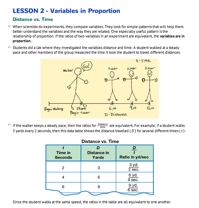
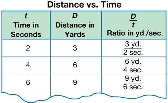
Introduce Distance vs. Time. Read together the narrative in the Distance vs. Time section of the Variables in Proportion pages of the Student Guide. Here the concept of a variables in proportion is illustrated with a Distance vs. Time experiment. Two variables are in proportion when their ratios are equivalent. Display the Distance vs. Time data table shown in Figure 1.

Ask:

What patterns do you see with the ratios D/t? (Possible responses: The yards are increasing by 3 and the seconds are increasing by 2; the D/t ratios 9/6 and 6/4 can both be reduced to 3/2.)
What would be the next ratio in the sequence? (12/8)
How do you know the ratios are equivalent (Question 1)? (Possible response: Each ratio in the table is equivalent to 3 yards/2 seconds.)

Have each student graph the variables listed on the data table using Centimeter Grid Paper (Question 2A). Then put students in pairs to describe and discuss their graph (Question 2B). Walk around and observe student work. Choose one student pair to draw the graph on the display and share their description.

Students should note that the graph is a straight line that goes uphill. The line meets the vertical axis at (0 s, 0 yd). When variables are in proportion to one another, the resulting graph is a straight line through the origin. Figure 2 shows a sample graph.

For Question 3, students choose two points on the line and write ratios corresponding to these points. Have student pairs come up to the display to share some of their examples. Two points are circled on the line in Figure 2 and the ratios corresponding to these points are shown. These two ratios are equivalent: 3 yards /2 seconds = 12 yards/8 seconds.

Use Questions 4–6 to explore the relationship between variables in proportion. If you double or triple one of the variables in proportion, the other variable will double or triple as well (Questions 4A–B). Using examples from Distance vs. Time, if a student walks 3 yards every 2 seconds, then he or she will walk 6 yards in 4 seconds and 9 yards in 6 seconds. In fact, if you multiply one variable by any number, the other variable will be increased by the same factor (Question 4C). This can be shown using equivalent fractions:

3 yd./2 sec. = 3 yd. × 4/2 sec. × 4 = 12 yd./8 sec.

For Question 5, students find the average distance walked in one second, the unit ratio. Dividing 3 yards by 2 seconds, students find that the walker averages 1.5 yards per second. Writing the D/t as a unit ratio is one strategy for solving distance problems. Since we know how far the walker travels in one second, we can multiply to find out the distance the walker traveled in any number of seconds.

In time calculations, the word per is often used. Per means “for each.” When a car drives 55 miles per hour, it is driving 55 miles for each hour on the road. In other words, if you drove 165 miles in 3 hours, it would not likely be written “165 miles per 3 hours,” but “55 miles per hour.” Use the word per frequently so students become accustomed to it.

For Question 6, students show how they can find the distance traveled if they know how long the student walked. Using the unit ratio is one way to answer this question. Encourage students to look for other strategies using patterns in the data table moving across the rows, and patterns using multiplication or division. Possible responses include:

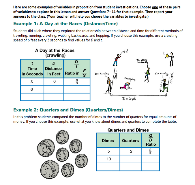
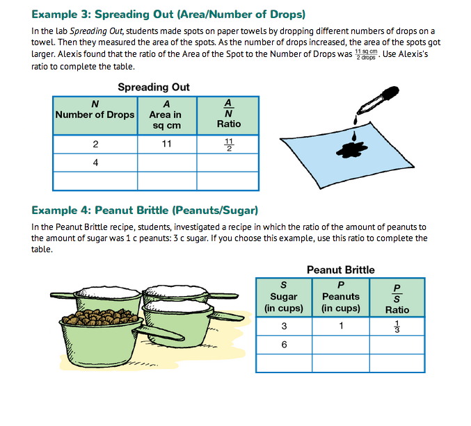
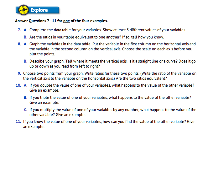
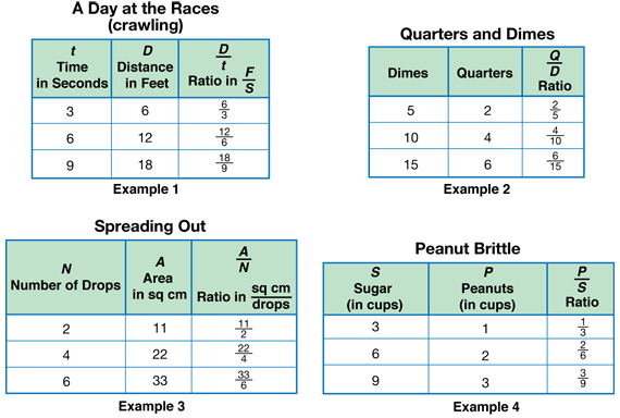
Explore Variables in Proportion. Read together the four examples of variables in proportion. Have students explore the proportional relationship between the variables involved. Assign one example to each group to make sure each example is investigated. Students work in groups to answer Questions 7–11 using their examples. Groups will then share their results with the class.

Questions 7–11 are similar to Questions 1–6. Students complete a data table, draw a graph, and write a proportion that is true for the variables. Completed tables are shown in Figure 3 and completed graphs are shown in Figure 4.

Be sure students write the ratio as given, with the variable from the first column in the denominator and that from the second column in the numerator, and not the other way around. This order is used so that when the data are graphed, in keeping with the convention that the first column variable goes on the horizontal axis, then this ratio corresponds to the steepness or slope of the line. The steeper the line, the greater the ratio. This will be useful in situations where we want to compare ratios, for instance, in the Mass vs. Volume: Proportions and Density lab in Lesson 4.

Report Result. After they have answered Questions 7–11, have each group report their results to the class. By discovering the common results for different pairs of variables in proportion, students will be able to generalize what they have learned and apply this knowledge to solve other problems. Use the following discussion prompts to help guide class discussion.

Ask:

How can you show that all of the ratios in your table are equal to one another (Question 7B)? (One way is to reduce all the fractions to lowest terms.)
How are the graphs alike (Question 8)? (All of the graphs are straight lines that go through the point (0, 0). All of the graphs go up as you read from left to right.)
If you double or triple the value of one of your variables, what happens to the other variable (Questions 10A–10B)? (For all pairs of variables that are in proportion, doubling or tripling one variable will double or triple the other. For instance, in Example 4 if you double the number of cups of peanuts in the peanut brittle recipe, you must also double the number of cups of sugar.)
If you multiply one of your variables by any number, what happens to the other variable (Question 10C)? (If you multiply one of the variables by a number, the other variable increases by the same factor. So, if you are making a very large batch of peanut brittle in which the ratio of peanuts to sugar is 1/3, then if you use 10 cups of peanuts, you must use 10 × 3 or 30 cups of sugar.)
How can you find one variable if you know the value of the other variable (Question 11)? (Variables in proportion are always related by multiplication. I look for patterns across the rows in the data tables.)

In Example 1, students can find the distance by multiplying the time by 2: D = 2 × t. That is, if a student crawls for 9 seconds, we know that he or she will travel 2 × 9 or 18 yards. In Example 2, we can find the number of dimes equal in value to any number of quarters by multiplying the number of quarters by 21/2: D = 21/2 × Q. The value of 10 quarters is the same as the value of 21/2 × 10 or 25 dimes.

Often, finding the unit ratio is helpful. In Example 3, the ratio of area to number of drops in the Spreading Out experiment is 11 sq cm to 2 drops. Dividing 11 by 2, we can write the ratio as 5.5 sq cm/1 drop. Knowing the area covered by 1 drop allows us to find the area for any number of drops.

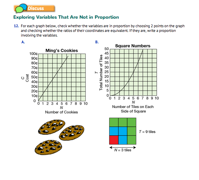
Explore Variables That Are Not in Proportion. Not all variables in experiments are in proportion. In Question 12, students examine graphs of several variables.

Ask:

Are the graphs familiar? Tell the story of each graph.

Graph A shows that as the number of cookies increases, the cost of the cookies increases as well.

Graph B shows the number of tiles along the side of a square and the number of tiles in the whole square. The resulting graph has a curved line.

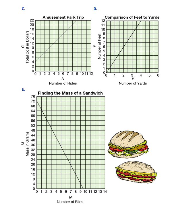
Graph C shows the total cost of going to an amusement park if the cost of admission into the park is $4 and each ride costs $2.

Graph D can be used as a tool for changing feet to yards and yards to feet.

Graph E shows how the mass of a sandwich decreases as students take bites out of it.

Students use the graphs to find out if the variables in each graph are in proportion. The variables in Graphs A and D are in proportion. However, the variables in Graphs B, C, and E are not. If the variables are in proportion, we can choose two points from the graph, write ratios corresponding to these two points, and see that the two ratios are equal. For example, to find out if the variables in Graph A are proportional, consider the points (2 cookies, 30¢) and (4 cookies, 60¢). The ratios 30 ¢/2 cookies and 60¢/4 cookies are equivalent fractions. In fact, any other point on the line would have a ratio equivalent to 15¢/1 cookie. (Students can choose other points until they are convinced of this.) Therefore, the variables number of cookies (N) and cost (C) are in proportion and a proportion between them is expressed by C/N = 15¢/1 cookie.

The variables in Graph B are not in proportion. Consider the points (4, 16) and (5, 25) or any other pair of points on the graph. The ratios 16/4 and 25/5 are not equivalent. Therefore, the variables on this graph are not in proportion. Similar comparisons for the other graphs will help the students determine which graphs represent variables in proportion.

Rather than checking for a proportion, we can quickly tell whether variables are in proportion or not by examining their graphs. In Question 13, students should look back over their graphs to find what features are shared by graphs of variables in proportion. Graphs A and D, which represent variables in proportion, are both straight lines and they both include the origin (0, 0). In fact, any graph that is a straight line graph through (0, 0) represents variables in proportion and any graph that is not represents variables that are not in proportion.

Question 14 asks students to choose a graph from Question 12 that represents variables that are not in proportion and examine the multiplication property they explored in Question 10. Use Graph E, for example, and choose a value of N = 4 bites. Using the graph, we see that after 4 bites were taken from the sandwich, the mass of the sandwich was 42 grams (M = 42 grams). If we double the number of bites (N = 8 bites), then we see from the graph that the mass of the sandwich is only 12 grams (M = 12 grams). Obviously, doubling the number of bites did not double the mass of the sandwich. Therefore, the variables N and M are not in proportion.

Use Graphs to Solve Variables in Proportion Problems. Graphs are useful because they display the relationship between the variables. When the variables are in proportion, the data points lie on a straight line, and we can use that line to make very good predictions. In Questions 15–16, students use graphs of variables in proportion to solve problems. The skills practiced here can be applied again in the lab Mass vs. Volume in Lesson 4 and in any other situation where the graph is a straight line through (0, 0). This type of graph is very common; students should be reminded, however, that the techniques will not work for other types of graphs.

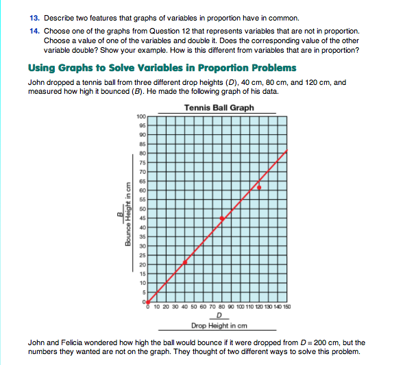
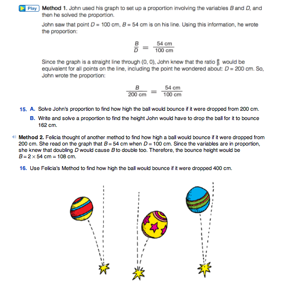
Read together the beginning of this section in which John's bouncing ball problem is described. For students who have not done the experiment, illustrate it by dropping a ball from different heights. Students should see that the higher the drop height, D, the higher the bounce height, B. The relationship between D and B for John's tennis ball is shown on the graph. In Question 15A students solve the proportion using Method 1.

The denominator on the left-hand side is twice the denominator on the right-hand side. Because the ratios are equivalent, the numerators should have the same relationship. Therefore, B = 2 × 54 cm = 108 cm.

In Question 15B, students write and solve the proportion:

Here, the numerator on the left-hand side is three times that on the right-hand side, and because the ratios are equivalent, the denominators are related the same way. This means D = 3 × 100 cm = 300 cm. If students do not observe that one numerator is three times the other, they can determine the factor relating the numerators by dividing: 162 ÷ 54 = 3, so 162 is 3 times 54.

In Question 16, students use a related method, Method 2, to find how high the ball would bounce if it were dropped 400 cm. D = 400 cm is not on the graph, but D = 100 cm is on the graph. A ball dropped from D = 100 cm bounces B = 54 cm. Therefore, a ball dropped from 4 times that height, D = 400 cm, would bounce 4 times that amount, B = 4 × 54 cm = 216 cm. Remind students that this method works because D and B are in proportion, as they can see from the graph, which is a straight line through (0, 0). This method is an application of the fact they observed in Question 10 that multiplying one variable results in the multiplication of the other by the same factor. As they observed in Question 14, this method does not work if the variables are not in proportion.

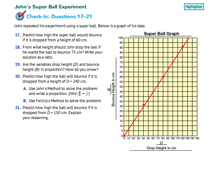
Use Check-In: Questions 17–21 in the John's Super Ball Experiment section to assess students' progress in identifying whether or not variables are in proportion, representing the relationship between variables as a ratio, using ratios and proportions to solve problems, and using patterns in tables and line graphs to make predictions and solve problems.

Use students' responses to Check-In: Questions 17–21 in the Student Guide to assess their abilities to represent the relationship between variables as a ratio [E2]; use ratios and proportions to solve problems [E4]; and use patterns in tables and line graphs to make predictions and solve problems [E12].

For Questions 17–18, students read the Super Ball Graph to solve problems finding drop and bounce height. For Question 19, students identify whether or not the variables for the Super Ball Graph are in proportion and explain how they know. For Question 20–21, students use Felicia and John's methods to predict how high the ball will bounce if it is dropped from a height of D = 240 cm and D = 150 cm.